Aims of the chapter

This chapter examines the implications on economic growth of technological progress, which was the crucial element missing in the basic version of the Solow model described in the previous chapter. The first part of the chapter assesses the strengths and main limitations of the Solow model augmented by exogenous technological progress. The second part of the chapter revises the theoretical underpinnings of endogenous growth models, to highlight the importance of institutional factors, education, and macroeconomic policy for the long-run growth rate of GDP per worker, therefore providing more plausible and comprehensive explanations of the cross-country and intertemporal differences in economic growth observed in the data.

• explain the effect of technological progress on economic growth
• discuss and interpret the Solow residual
• illustrate the main assumptions and motivations of the Solow model with exogenous technological progress, and describe the behaviour of the economy in the short and long run
• critically analyse the main limitations of exogenous models of economic growth
• describe the theoretical underpinnings of endogenous growth models.

The basic Solow model, described in the previous chapter of the guide, predicts that output and consumption per worker should not grow in the
long run. This contradicts the persistent growth observed in industrialised countries, as reported by Kaldor’s first stylised fact. The crucial omission in this basic version of the Solow model is the role of technological progress in economic growth, which is the central topic of this chapter of the guide. We begin by revising the alternative ways of introducing technological progress into the aggregate production function, and describe how the so-called Solow residual is employed by economists to account for the contribution to economic growth of the growth in factors different from capital and labour.

Next, we recast the whole analysis of the Solow model by adding to the production function a labour-augmenting technology, which grows over time at a constant and exogenous positive rate. The most appealing feature of this new model is that it can explain the sustained growth observed in most industrialised countries over the last 60 years. However, the model is silent about the sources of technological progress, it cannot explain why
technological progress may change over time, and it still predicts that the savings rate can only affect the level of GDP per worker, having no effect
on its growth rate.

The second part of the chapter focuses on models of economic growth in which technological progress is an endogenous variable determined within the model, to highlight the contribution of macroeconomic policy (particularly changes in the savings rate) and human capital accumulation on long-run economic growth. You are expected to be able to explain the motivations and policy implications of the new growth theory, as well as illustrating the basic analytical underpinnings of endogenous growth models.

Production with exogenous technology

The standard approach to introducing technological progress into the analysis of economic growth consists in postulating that the production function includes a so-called labour-augmenting technology parameter:
Y t = F ( K t , A t N t ), (6.1)

where A t indicates the level of technical progress. Since technology enters the production function in a multiplicative way through the variable
A t N t , the technology variable in equation (6.1) is also referred to as labour-augmenting or Harrod-neutral. 1 In addition, technology is assumed to grow over time at the constant rate g A :
A t = ( 1 + g A ) A t − 1 .

Assuming that the production function in equation (6.1) displays constant returns to scale, it is easy to show that it can be written as:

Yt/(At Nt) = f((Kt/(At Nt)) , or equivalently as: hat yt = f ( hat kt ),

where where haty t = Y t/ At Nt and hat k_t = Kt/AtNt indicate output and capital per effective worker, A t N t , respectively.

It is essential that you are aware of the link between variables measured in terms of ‘effective worker’ and variables measured in terms of ‘worker’. For example, output per effective worker is equal to:
Y t = y t/A t N A t

i.e. the ratio between output per worker and the level of technology). This is a crucial feature of the new model, because it implies that the growth rate of a variable measured per effective worker is always equal, by definition, to the growth rate of that variable measured in per-worker terms, minus the growth rate of technology. Thus the growth rate of output per effective worker is always equal to the growth rate of output per worker minus the growth rate of technology:

g_haty,t = g_y,t − g_A,t

The Solow residual

The Solow residual was devised by Robert Solow in 1957 in order to account for the contribution to the growth of output made by the growth of factor inputs, such as capital and labour, and to associate any growth unaccounted for with technological progress. Analytically, the Solow residual, R, is written as:

R = g Y − [ α g K + ( 1 − α ) g N ],

where g Y is the growth rate of GDP, g K is the growth rate of capital, g N is the labour force growth rate, and α is the share of capital in output, as measured by the standard Cobb–Douglas production function. 2 The Solow residual is sometimes interpreted as a measure of the contribution to growth of technological progress. However, as shown in its derivation, the Solow residual reflects all sources of growth other than the contribution of capital and labour. For this reason, the Solow residual is also called the **rate of growth of total factor productivity** (TFP). Measurements of the Solow residual indicate that technology is a very important factor in growth. For example, the empirical evidence in OECD countries shows that it has accounted for more than a half of GDP growth on average since the end of the Second World War. However, it is important that you bear in mind the main shortcomings of this measure of technological progress. The Solow residual is derived under the assumption that the production function exhibits constant returns to scale and markets are perfectly competitive. In addition, the standard derivation of the Solow residual assumes that aggregate output includes only three factors: capital, labour and technological progress, and thus it omits the contribution to growth arising from other factors, such as human capital and land.

The Solow model with exogenous technology

In the Solow model with exogenous technological progress the aggregate economy is entirely described by the following equations:

Income identity: Y t = C t + I t
Aggregate production (GDP): Y t = F (K t , A t N t )
Aggregate consumption: C t = (1 – s) Y t = (1 – s) F (K t , A t N t )
Investment: S t = sY t = sF (K t , A t N t ) = I t
Population growth: N t = (1 + g N )N t–1
Technological growth: A t = (1 + g A )A t–1
Capital accumulation: K t+1 – K t = sF (K t , A t N t ) – δK t .

The income identity states that, in a closed economy without a government sector, aggregate income equals the sum of aggregate consumption and investment in equilibrium. Aggregate production embodies a labour-augmenting technological progress, as described in the previous section, and it is assumed to retain all the properties of the neoclassical production function (CRTS, positive, but diminishing, marginal products of capital and effective labour, Inada conditions). Since the savings rate s is constant and exogenous, aggregate consumption is a constant fraction, 1–s, of aggregate income. Private saving equals investment and it is given by a fraction s of aggregate income. The labour force and technology change over time at the constant and exogenous rates g N and g A respectively. The capital stock changes over time as a result of gross investment, sF(K t , A t N t ), and physical depreciation, δK t .

The aggregate description of the model can be employed to derive in per-worker terms the equations for the three endogenous variables of the
Solow model with exogenous technological progress.

Output per effective worker is determined by dividing both sides of the aggregate production function by the effective worker term A t N t , which yields:

Yt/At Nt = F(Kt/(AtNt),1) <-> hatyt = f(hatkt) (6.2)

which holds under CRTS. Similarly, consumption per effective worker is given by dividing both sides of the aggregate consumption equation by the effective worker term A t N t , which yields:

Ct/AtNt = (1 - s )(Y/(AtNt)) = (1 - s) F((Kt, AtNt)/(AtNt)) or equivalently;
cˆt = ( 1 − s ) yˆt = ( 1 − s ) f ( kˆ t ).

To obtain the dynamic equation for capital accumulation in per-worker terms, start by dividing both sides of the corresponding aggregate equation by K t :

((K t+1 − K t) / K t) = s (F (K t , A t N t )/Kt) – δ
which is equivalent to:
((K t+1 − K t) / K t) = s (F (K t , A t N t )/Kt) ((AtNt)/(AtNt)) – δ
((K t+1 − K t) / K t) = s haty ( 1 / hatKt) - δ

This expression can be substituted into the formula for the growth rate of capital per effective worker, which is approximately equal to the difference between, on the one hand, the growth rate of capital and, on the other
hand, the sum of the growth rates of the labour force and technology, to obtain:

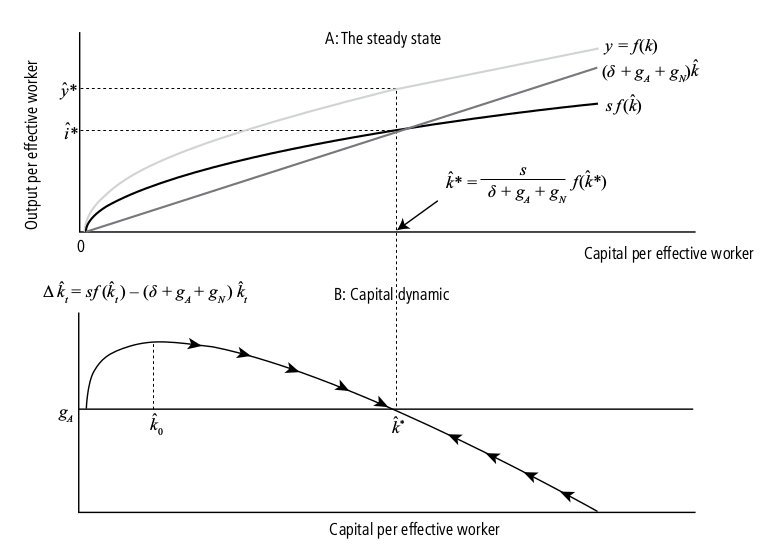
k ˆ t+1 − k ˆ t = sf ( k ˆ t ) − (δ + g A + g N ) k ˆ t

This dynamic equation of capital per effective worker also determines the evolution of output and consumption per effective worker over time. The term sf ( k ˆ ) measures actual investment per effective worker, (i.e. the quantity of resources devoted to the creation of new capital per effective worker). The term ( δ + g A + g N )k ˆ is break-even investment per effective worker, which measures the quantity of new investment required in each period of time in order to maintain a constant stock of capital per effective worker.

In the steady state the rate of growth of the endogenous variables c ˆ t , ˆ y t and k̂ t must be zero, by definition. That is, in steady state.

g yˆ = y ˆ t − yˆt − 1 / yˆ t = 0
g cˆ = c ˆ t − cˆt − 1 / cˆ t = 0
g kˆ = k ˆ t − kˆt − 1 / kˆ t = 0

The link between variables per effective worker and variables per worker
implies that at the steady state the following equalities hold:
g * y ˆ = g * y − g A = 0 ⇒ g * y = g A ,
g c *ˆ = g c * − g A = 0 ⇒ g c * = g A ,
g * k ˆ = g * k − g A = 0 ⇒ g * k = g A .

In other words, in the Solow model with exogenous technological progress, the long-run growth rates of output, consumption and capital per worker are all equal to the (exogenous) growth rate of technological progress. Consequently, in a Solow model with technological progress balanced growth occurs in the long run at a constant rate equal to the rate of growth of technological progress. Thus the new version of the Solow model implies that GDP per worker can permanently increase, but only because of an exogenous trend in technology. In turn, this shows that the predictions of the Solow model with exogenous technological progress are consistent with Kaldor’s first, second and fourth stylised facts listed in the previous chapter of the subject guide.

You can also view the basic version of the Solow model discussed in the previous chapter as a special case of the Solow model with exogenous technological progress, which is obtained by setting g A = 0 and A t =1 in equations (6.2), (6.3) and (6.4).

The steady state

We can now study the properties of the steady state in the Solow model with exogenous technological progress. In steady-state k ˆ t + 1 − k ˆ t = 0 , and the steady-state stock of capital per effective worker, k ˆ * , can be obtained by imposing this in equation (6.4):

sf ( k ˆ ) = ( δ + g + g ) k ˆ*, k ˆ * = (s/(δ + g A + g N)) f ( kˆ* ) .

The equation of capital per effective worker in (6.4) can be employed to assess the dynamic behaviour of the economy, which is fundamentally consistent with that of the basic Solow model described in the previous
chapter

If the stock of capital per effective worker is larger than its steady-state value,

k ˆ t < (s / (δ + g A + g N)) y ˆ * ,

actual investment per effective worker is lower than break-even investment per effective worker, sf ( k ˆ t ) < ( δ + g A + g N ) k ˆ t , and the economy is reducing its capital stock per effective worker, k ˆ t + 1 − k ˆ t < 0. Consequently, the growth rates of both capital and GDP per effective worker must be negative, g k ˆ > 0 and g y ˆ > 0 .

It is essential that you understand the dynamic behaviour of output and capital per worker while the stock of capital per effective worker changes
over time. Consider, for example, what happens to output per worker when the economy is accumulating capital per effective worker. The growth rate
of output per effective worker is positive, g y ˆ > 0 . Since the growth rate of technological progress is positive by assumption, the result is that:
g y,t = g y,tˆ + g A > 0 > 0

which shows that output per worker grows at a rate greater than the technological progress whenever g y,t ˆ > 0. In other words, in the Solow model with exogenous technological progress:

1. If actual investment per effective worker exceeds break-even investment per effective worker, sf ( k ˆ t ) > ( δ + g A + g N ) k ˆ t , both output and capital per worker are growing faster than the rate of technological progress, g y,t > g A and g k,t > g A .

2. If the stock of capital per effective worker is falling, both output and capital per worker are growing at lower rates than the rate of technological progress, g y,t < g A and g k,t < g A . Consequently, the Solow model with technological progress predicts that in the long run the economy always converges towards the level of GDP per effective worker in equation (6.5)

Figure 6.1 provides a graphical illustration of the Solow model with exogenous technological progress. Note how all variables are now measured in effective worker terms. Panel A plots output, actual investment and break-even investment per effective worker in capital-output per effective worker space. Panel B shows the dynamic of capital per effective worker. In steady state, capital per effective worker does not grow, just as the growth rate of capital per worker was zero in steady state in the simple model without technological progress.

Comparative statics

Comparative statics can be carried out to assess short- and long-run effects of changes in the parameters of the Solow model with exogenous technological progress.

Since the long-run growth rate of GDP per worker depends only upon the growth rate of technological progress, temporary and permanent changes in all parameters of the model, except for g A , can only have a temporary effect on the growth rate of GDP per worker. For example, an increase in the savings rate makes GDP per worker increase faster than g A , but only in the short run. In the long run, the higher savings rate cannot sustain growth in GDP per worker higher than g A .

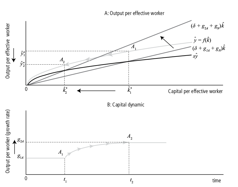
In turn, a permanent change in the growth rate of technological progress can permanently alter the rate of growth of GDP per worker, as illustrated in Figure 6.2. The effect of an increase in the growth rate of technological progress on output per effective worker is illustrated in Panel A. The economy is assumed to be in long-run equilibrium with the stock of capital per effective worker given by k ˆ 1 * . The rise in technological progress makes the break-even investment per effective worker line steeper, leaving the curves of output and actual investment per effective worker unaffected.

This implies that capital and output per effective worker converge to a lower steady state. The fall in output and capital per effective worker occurs because at the initial steady-state capital stock, k ˆ 1 * , there is insufficient investment per effective worker to keep capital per effective worker constant, given the faster growth in the number of effective workers caused by faster growth in technology. As a result, capital per effective worker must decrease to the lower level k ˆ 2 * .

Panel B illustrates the effect of a permanent increase in the growth rate of technological progress on the growth rate of output per worker. In the initial steady-state output per effective worker is constant by definition, whereas output per worker is growing at the rate g 1A . A permanent increase in the growth rate of technological progress to g 2A > g 1A has the effect of increasing the growth rate of output per worker, both in the short and in the long run, as depicted in Panel B. Note that after the technological improvement the growth rate of output per worker is given by: g y,t = g ŷ,t + g 2A > g 1A .

In the short run g ŷ,t is negative, gradually increasing to zero in the long run. Thus the growth rate of output per worker must gradually increase towards the higher rate of technological progress in the long run.

The golden rule

The Solow model with exogenous technological progress can be employed to compute the golden rule (GR) level of capital per effective worker, (i.e.
the steady-state stock of capital per effective worker that maximises long-run consumption). By definition, steady-state consumption is given by:
c ˆ = f ( k ˆ ) − ( δ + g A + g N ) k ˆ ,

and the GR level of capital per effective worker is obtained from the solution to the following optimisation problem:

max(hatk^GR) hatc^* = f ( kˆ^GR ) − ( δ + g A + g N ) kˆ^GR ,

which yields the GR condition: f ' ( k ˆ GR ) = δ + g A + g N .

In other words, the GR level of capital per effective worker is obtained when the marginal product of capital per effective worker equals the sum of the physical capital depreciation rate, and the growth rates of, technological progress and the labour force.

To get further insight into this result, consider the case of a Cobb–Douglas production function, so that f ( k ˆ ) = k ˆ α . The golden rule level of capital per effective worker is given by: α (k ˆ GR ) α–1 = δ + g A + g N , which can be solved for GR k ˆ as:

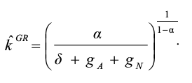
Figure 6.3 illustrates the golden rule equilibrium in the Solow model with exogenous technological progress. The figure shows that at the GR level of capital per effective worker the slope of the production function equals that of the break-even line for investment per effective worker. This ensures that the GR level of capital per effective worker maximises the steady-state level of consumption per effective worker.

New growth theory

The Solow model extended for technological progress, presented in this chapter of the subject guide, is an exogenous model of economic growth. There are two ways of looking at exogenous growth. First, the growth rate of technological progress is taken as given rather than being determined from other variables in the model. The technology level A t is an exogenous variable that grows at a constant rate g A : neither A t nor g A depend upon other variables in the model. Second, economic growth is exogenous in the Solow model in the sense that policy-makers cannot permanently affect the growth rate of GDP per worker in a country. This occurs because the long-run growth rate of output per worker is equal to the exogenous growth rate of technological progress.

In particular a policy that increases the private savings rate results only in a short-run increase in the growth rate of GDP per worker, having no effect in the long run. In other words, a change in the saving rate has a permanent level effect but not a permanent growth effect on output and consumption per worker.

For example, under the Cobb–Douglas labour-augmenting production function, the equilibrium level of GDP per worker is given by:

which shows that an increase in s can raise the long-run level of GDP per worker. However, the increase in the savings rate has no growth effect in the long run, even if growth does change initially. Remember that the short-run growth rate of GDP per worker is:

g y = g A + g y ˆ , with g y ˆ ≠ 0 ,

whereas the long-run rate of growth of GDP per worker is:
g y = g A .

Hence, the increase in s raises g y ˆ temporarily, but it has no effect in the long run since the steady-state growth rate of output per effective worker, g y ˆ , is always zero.

Another issue with the Solow model extended for exogenous technological progress is that it explains cross-country differences in average growth rates entirely in terms of differences between growth rates in technological progress. However, if technology is the outcome of knowledge and new ideas, which should, in principle, be non-rival goods accessible to all, the model cannot explain why several South American and African countries (which have not been growing over the last 50 years) have not had access to the same technology that has been driving economic growth in OECD countries.

Furthermore, the empirical evidence shows that the average growth rate has been changing over time even in industrialised countries. The Solow model with exogenous technological progress cannot explain why technology has been changing over different periods of time.

These fundamental weaknesses in the Solow model have been the driving force behind the development of ‘new growth theory’ since the beginning
of the 1980s. This new growth theory develops endogenous models of economic growth, in other words models in which:
i. technological progress is dependent upon other variables in the model, rather than being an exogenous process, and
ii. changes in the savings rate can have growth effects on GDP per worker.

From a technical point of view, an endogenous model of economic growth – a model in which policy can affect long-run growth – can be designed by appropriately modifying the production function. This task can be accomplished in two ways. The first approach consists of abandoning the assumption of diminishing returns to capital per worker, which prevents policy from being effective in the long run. This approach is at the basis of Romer’s AK model of economic growth.

There are other ways of designing an endogenous model of economic growth. For example, one could include human capital (H) as well as physical capital in the production function for aggregate output. This second approach underpins the so-called two-sector models, which study how research and development activities, education, and more generally improvements in the quality of the labour force, contribute to explain long-run growth, as well as intertemporal and cross country differences in growth rates.

The AK model

To understand the theoretical underpinnings of the first category of endogenous growth models, suppose GDP is produced by a Cobb–Douglas production function and consider the growth rate of capital per worker in the Solow model without technological progress:

k t+1 – k t/k t = g k = sk α–1 – (δ +g N )

We know that the stock of capital per worker increases if g k > 0 , which occurs when the actual stock of capital per worker is lower than the steady state, k t < k * . Under the standard assumption α < 1, the production function displays diminishing returns to capital per worker. This means that the more capital per worker there is, the lower is the term sk α−1 : eventually growth in k causes g k to fall to zero, and a steady state is
reached.

Suppose instead that the production function displays constant (rather than diminishing) returns to capital per worker, so that α = 1 and y t = k t . This implies that the growth rate of capital per worker is given by:

g k = s – (δ + g N ).

Thus, economic growth occurs whenever the private savings rate is greater than the growth rate of the labour force plus physical depreciation:
s > δ + g N .

This simple example shows that an endogenous model of economic growth can be obtained by assuming that the production function displays constant returns to capital per worker, without considering technological progress. This model of growth is endogenous because a change in the savings rate has a permanent effect on the growth rate of capital per effective worker.

By way of analogy, in the Solow model with exogenous technology the growth rate of capital per worker is given by:

k ˆ t + 1 − k ˆ t/k ˆ = g k ˆ = s k ˆ t − ( δ + g A + g N ).

If the production function displays constant, rather than decreasing, returns to capital per effective worker, then y ˆ t = k ˆ t , and the growth rate of capital per effective worker is given by:
g k ˆ = s − ( δ + g A + g N ).

In this model persistent growth in GDP per worker at a positive rate higher than g A can be obtained whenever the savings rate satisfies:

s > δ + g A + g N .

Growth and human capital

An endogenous model of economic growth can be designed by including human capital (H) instead of labour in the production function for aggregate output:

Y t = F ( K t , H t )

The function F is assumed to have CRTS in K t and H t , so that output per worker can be written as:

Yt/Nt = F ((Kt/Nt)(Ht/Nt))

If h t = Ht/Nt then an intensive form of the production function can be written as: y t = f ( k t , h t ). Where f(k t ,h t ) equals F(k t ,h t ). Consider the case of a Cobb–Douglas production function: y t = k α t h t 1– α ,

so that the production function displays CRTS and diminishing returns to capital per worker. Now, suppose that as a result of an increase in the savings rate both physical and human capital rise by a factor μ > 0. CRTS
implies that:
(μk t ) α (μh t ) 1– α = μ α k t α μ 1– α h 1– t α = μ k t α h 1– t α = μy t ,

which shows that if saving can induce the accumulation of human as well as physical capital, then an increase in the savings rate can permanently raise output per worker.

This is the main insight behind endogenous models of economic growth based on a production function which includes human capital as well as physical capital, and displays constant returns to these two factors.

Blanchard, O., Johnson, D.R., (2013) Macroeconomics (sixth edition), Pearson

Chapter 12: Technological Progress and Growth

**12-1 Technological Progess and the Rate of Growth**

The state of technology is a variable that tells us how much output can be produced from given amounts of capital and labor at any time. If we denote the state of technology by A, we can rewrite the production function as

Y = F (K, N, A)

Given capital and labor, an improvement in the state of technology, A, leads to an increase in output.

Technological progress reduces the number of workers needed to produce a given amount of output. Doubling A produces the same quantity of output with only half the original number of workers, N.

Technological progress increases the output that can be produced with a given number of workers. We can think of AN as the amount of effective labor in the economy. If the state of technology A doubles, it is as if the economy had twice as many workers. In other words, we can think of output being produced by two factors: capital (K ), and effective labor (AN ). AN is also sometimes called labor in efficiency units.

It is reasonable to assume constant returns to scale: For a given state of technology (A): xY = F (xK, xAN)

It is also reasonable to assume decreasing returns to each of the two factors—capital and effective labor. Given effective labor, an increase in capital is likely to increase output, but at a decreasing rate.

It is convenient here to look at output per effective worker and capital per effective worker. In steady state, output per effective worker and capital per effective worker are constant.

To get a relation between output per effective worker and capital per effective worker, take x = 1/AN. This gives:

Y/AN = F(K/AN, 1) . Or, if we define the function f so that f(K/AN) := K F(K/AN, 1); Y/AN = f(K/AN)

Output per effective worker (the left side) is a function of capital per effective worker (the expression in the function on the right side).

Because of decreasing returns to capital, increases in capital per effective worker lead to smaller and smaller increases in output per effective worker.

Investment is equal to private saving, and the private saving rate is constant—investment is given by: I = S = sY

I/AN = sY/AN

Replacing output per effective worker, Y>AN, by its expression from equation. I/AN = sf(K/AN)

Capital per effective worker and output per effective worker converge to constant values in the long run.

The steady state of this economy is such that capital per effective worker and output per effective worker are constant and equal to (K/AN)* and (Y/AN)2* , respectively.

This implies that, in steady state, output 1Y 2 is growing at the same rate as effective labor 1AN 2 (so that the ratio of the two is constant). Because effective labor grows at rate (g_A + g_N), output growth in steady state must also equal (g_A + g_N_. The same reasoning applies to capital. Because capital per effective worker is constant in steady state, capital is also growing at rate (gA + gN).

If Y/AN is constant, Y must grow at the same rate as AN. So, it must grow at rate g_A + g_N

In steady state, the growth rate of output equals the rate of population growth 1g N 2 plus the rate of technological progress 1g A 2. By implication, the growth rate of output is independent of the saving rate.

In the absence of technological progress and population growth, the economy could not sustain positive growth forever. Suppose the economy tried to sustain positive output growth. Because of decreasing returns to capital, capital would have to grow faster than output. The economy would have to devote a larger and larger propor- tion of output to capital accumulation. At some point there would be no more output to devote to capital accumulation. Growth would come to an end; same applies to labour.

**When the economy is in steady state, output per worker grows at the rate of technological progress. The steady state of this economy is also called a state of balanced growth**

On the balanced growth path (equivalently: in steady state; equivalently: in the long run):

* Capital per effective worker and output per effective worker are constant.
* Equivalently, capital per worker and output per worker are growing at the rate of technological progress, g_A .
* Or, in terms of labor, capital, and output: Labor is growing at the rate of population growth, g_N ; capital and output are growing at a rate equal to the sum of population growth and the rate of technological progress, (g_A + g N 2.

An increase in the saving rate leads to an increase in the steady-state levels of output per effective worker and capital per effective worker.

In steady state, the growth rate of output depends only on the rate of population growth and the rate of technological progress. Changes in the saving rate do not affect the steady-state growth rate. But changes in the saving rate do increase the steady-state level of output per effective worker.

The increase in the saving rate leads to higher growth until the economy reaches its new, higher, balanced growth path.

Summarize: In an economy with technological progress and population growth, output grows over time. In steady state, output per effective worker and capital per effective worker are constant. Put another way, output per worker and capital per worker grow at the rate of technological progress. Put yet another way, output and capital grow at the same rate as effective labor, and therefore at a rate equal to the growth rate of the number of workers plus the rate of technological progress. When the economy is in steady state, it is said to be on a balanced growth path. The rate of output growth in steady state is independent of the saving rate. However, the saving rate affects the steady-state level of output per effective worker. And increases in the saving rate lead, for some time, to an increase in the growth rate above the steady-state growth rate.

**12-2 The Determinants of Technological Progress**

Firms spend on R&D for the same reason they buy new machines or build new plants: to increase profits. By increasing spending on R&D, a firm increases the probability that it will discover and develop a new product.

The fertility of research depends on the successful interaction between basic research (the search for general principles and results) and applied research and development (the application of these results to specific uses, and the development of new products). Basic research does not lead, by itself, to technological progress. But the success of applied research and development depends ultimately on basic research.

The second determinant of the level of R&D and of technological progress is the degree of appropriability of research results. If firms cannot appropriate the profits from the development of new products, they will not engage in R&D and technological progress will be slow. Even more important is the legal protection given to new products. Without such legal protection, profits from developing a new product are likely to be small. Too little protection will lead to little R&D. Too much protection will make it difficult for new R&D to build on the results of past. R&D, and may also lead to little R&D.

**12-3 The Facts of Growth Revisited**

Suppose we observe an economy with a high growth rate of output per worker over some period of time. Our theory implies this fast growth may come from two sources:

* It may reflect a high rate of technological progress under balanced growth.
* It may reflect instead the adjustment of capital per effective worker, K/AN, to a higher level. As we saw in Figure 12-4, such an adjustment leads to a period of higher growth, even if the rate of technological progress has not increased.

Can we tell how much of the growth comes from one source and how much comes from the other? Yes. If high growth reflects high balanced growth, output per worker should be growing at a rate equal to the rate of technological progress. If high growth reflects instead the adjustment to a higher level of capital per effective worker, this adjustment should be reflected in a growth rate of output per worker that exceeds the rate of technological progress.

The growth since 1985 has come from technological progress, not unusually high same rate over this period. This conclusion follows from the fact that, in all four countries, the growth rate of output per worker has been roughly equal to the rate of technological progress. This is what we would expect when countries are growing along their balanced growth path.

The nature of technological progress is likely to be different between more advanced and less advanced economies. The more advanced economies, being by definition at the technological frontier, need to develop new ideas, new processes, new products.

Dornbusch, R., S. Fischer and R. Startz Macroeconomics (2011)

Chapter 4 Growth and Policy

Highlights

• Rates of economic growth vary widely across countries and across time.
• Endogenous growth theory attempts to explain growth rates as functions of societal decisions, in particular saving rates.
• The role of human capital and investment in new knowledge is a key to endogenous growth theory.
• Income in poor countries appears to be converging toward income levels of rich countries, but at extremely slow rates.

Endogenous growth theory emphasizes different growth opportunities in physical capital and knowledge capital. There are diminishing marginal returns to the former, but perhaps not to the latter. The idea that increased investment in knowledge increases growth is a key to linking higher saving rates to higher equilibrium growth rates.

Neoclassical growth theory predicts absolute convergence for economies with equal rates of saving and population growth and with access to the same technology. In other words, they should all reach the same steady-state income.

Conditional convergence is predicted for economies with different rates of saving or population growth; that is, steady-state incomes will differ as
predicted by the Solow growth diagram, but growth rates will eventually equalize.

While countries that invest more tend to grow faster, the impact of higher investment on growth seems to be transitory: 8 Countries with higher investment will end in a steady state with higher per capita income but not with a higher growth rate. This suggests that countries do converge conditionally, and thus endogenous growth theory is not very important for explaining international differences in growth rates, although it may be quite important for explaining growth in countries on the leading edge of technology.

Recap
• Endogenous growth theory relies on constant returns to scale to accumulable factors to generate ongoing growth.
• The microeconomics underlying endogenous growth theory emphasizes the difference between social and private returns when firms are unable to capture some of the benefits of investment.
• Current empirical evidence suggests that endogenous growth theory is not very important for explaining international differences in growth rates.

SUMMARY
1. Economic growth in the most developed countries depends on the rate of technological progress. According to endogenous growth models, technological progress depends on saving, particularly investment directed toward human capital.
2. International comparisons support conditional convergence. Adjusting for differences in saving and population growth rates, developing countries advance toward the income levels of the most industrialized countries.
3. There are extraordinarily different growth experiences in different countries. High saving, low population growth, outward-looking orientation, and a predictable economic environment are all important progrowth factors.

Mankiw, N. G. Macroeconomics. (Worth, 2009)

Chapter 8: Economic Growth II: Technology, Empirics, and Policy

In Chapter 7 we developed the Solow model to show how changes in capital (through saving and investment) and changes in the labor force (through population growth) affect the economy’s output. We are now ready to add the third source of growth—changes in technology—to the mix. The Solow model does not explain technological progress but, instead, takes it as exogenously given and shows how it interacts with other variables in the process of economic growth.

According to the Solow model, only technological progress can explain sustained growth and persistently rising living standards.

Steady-State Growth Rates in the Solow Model With Technological Progress

Variable Symbol Steady-State Growth Rate
Capital per effective worker k = K/(E × L) 0
Output per effective worker y = Y/(E × L) = f(k) 0
Output per worker Y/L = y × E g
Total output Y = y × (E × L) n+g

The introduction of technological progress also modifies the criterion for the Golden Rule. The Golden Rule level of capital is now defined as the steady state that maximizes consumption per effective worker.

According to the Solow model, technological progress causes the values of many variables to rise together in the steady state. This property is called balanced growth.

The Solow model’s prediction about factor prices—and the success of this prediction—is especially noteworthy when contrasted with Karl Marx’s theory of the development of capitalist economies. Marx predicted that the return to capital would decline over time and that this would lead to economic and political crisis. Economic history has not supported Marx’s prediction, which partly explains why we now study Solow’s theory of growth rather than Marx’s.

Summary
1. In the steady state of the Solow growth model, the growth rate of income per person is determined solely by the exogenous rate of technological
progress.
2. Many empirical studies have examined to what extent the Solow model can help explain long-run economic growth. The model can explain much of what we see in the data, such as balanced growth and conditional convergence. Recent studies have also found that international variation in standards of living is attributable to a combination of capital accumulation and the efficiency with which capital is used.
3. In the Solow model with population growth and technological progress, the Golden Rule (consumption-maximizing) steady state is characterized
by equality between the net marginal product of capital (MPK − ) and the steady-state growth rate of total income (n + g). In the U.S. economy, the
net marginal product of capital is well in excess of the growth rate, indicating that the U.S. economy has a lower saving rate, indicating that the U.S. economy has a lower saving rate and less capital than it would have in the Golden Rule steady state.
4. Policymakers in the United States and other countries often claim that their nations should devote a larger percentage of their output to saving and investment. Increased public saving and tax incentives for private saving are two ways to encourage capital accumulation. Policymakers can also
promote economic growth by setting up the right legal and financial institutions so that resources are allocated efficiently and by ensuring proper
incentives to encourage research and technological progress.
5. In the early 1970s, the rate of growth of income per person fell substantially in most industrialized countries, including the United States. The cause of this slowdown is not well understood. In the mid-1990s, the U.S. growth rate increased, most likely because of advances in information technology.
6. Modern theories of endogenous growth attempt to explain the rate of technological progress, which the Solow model takes as exogenous. These models try to explain the decisions that determine the creation of knowledge through research and development.

Appendix: Accounting for the Sources of Economic Growth

Increases in the Factors of Production

Start by assuming there is no technological change, so the production function relating output Y to capital K and labor L is constant over time:

Y = F(K, L).

In this case, the amount of output changes only because the amount of capital or labor changes.

Increases in Capital First, consider changes in capital. If the amount of capital increases by ΔK units, by how much does the amount of output increase? To answer this question, we need to recall the definition of the marginal product of capital MPK:

MPK = F(K + 1, L) − F(K, L).

The marginal product of capital tells us how much output increases when capital increases by 1 unit. Therefore, when capital increases by ΔK units, output increases by approximately MPK × ΔK.

For example if the Marginal Product of Kapital (MPK) is 1/5, the addition of 10 unites of Kapital will increase Y by 2 units.

Exactly the same reasoning can apply to Labour, Marginal Product of Labour (MPL)

Increases in Capital and Labor

ΔY = (MPK × ΔK ) + (MPL × ΔL)

Following this measurement of change, we can build the growth rate.

ΔY/Y = (MPK × K/ Y )ΔK/K + (MPL × L)ΔL/L

Next, we need to find some way to measure the terms in parentheses in the last equation. The marginal product of capital equals its real rental price. Therefore, MPK × K is the total return to capital, and (MPK × K )/Y is capital’s share of output. Similarly, the marginal product of labor equals the real wage. Therefore, MPL × L is the total compensation that labor receives, and (MPL × L)/Y is labor’s share of output. Under the assumption that the production function has constant returns to scale, Euler’s theorem tells us that these two shares sum to 1. Therefore

ΔY/Y = alpha(ΔK/K) + (1 - alpha)(ΔL/L)

We include the effects of the changing technology by writing the production function as

Y = AF(K, L)

Which now generates

ΔY/Y = alpha(ΔK/K) + (1 - alpha)(ΔL/L) + (ΔA/A)

Growth in output = Growth of Kapital share + Growth of Labour share + Growth of Total Factor Productivity (Technology)

Technologies contribution is measured:

(ΔA/A) = ΔY/Y - alpha(ΔK/K) - (1 - alpha)(ΔL/L)

Total factor productivity can change for many reasons. Changes most often arise because of increased knowledge about production methods, so the Solow residual is often used as a measure of technological progress. Yet other factors, such as education and government regulation, can affect total factor productivity as well. For example, if higher public spending raises the quality of education, then workers may become more productive and output may rise, which implies higher total factor productivity. As another example, if government regulations require firms to purchase capital to reduce pollution or increase worker safety, then the capital stock may rise without any increase in measured output, which implies lower total factor productivity. *Total factor productivity captures anything that changes the relation between measured inputs and measured output*. (p250)